Is a neural network better than Ash at detecting Team Rocket? If so, how?
Training CNNs in TensorFlow, object detection models in Google Cloud, and visualizing activation maps in TensorFlow.js.

Our whole existence is a never-ending riddle. Are we the only ones in the Universe? What's the point of life? Is a neural network better than Ash at recognizing Team Rocket? The first two are non-trivial questions that keep many scientists and philosophers up at night. The last one, however, does not let me sleep. In this article, I'll attempt to answer it.
These days I've taken some of my lockdown time to watch the first season of the Pokemon show (it is not like I need an excuse anyway). As I watched Ash and Friends embark on their adventures capturing pocket monsters and becoming the very best (like no one ever was), I couldn't help noticing that they never recognize Team Rocket when they wear any of their iconic costumes. I mean, come on people, Team Rocket is always there, on every step of your journey, and you're telling me that you can't notice them? That's weird. But sure, that's ok; Pokemon world rules, I guess. But then, I thought, "hmmm wait a second, what about a neural network? Could a neural network be better than Ash & Crew at identifying Team Rocket?" Well, probably. But I don't have much to do these days, so let's see it in action. Besides, sometimes the journey is better than the destination.
Before continuing, for those of you who have no idea who Team Rocket is, it is a trio—consisting of Jessie, James, and Meowth—who plays the main antagonist of the Pokemon anime. Its main goal is to steal Pikachu from Ash. For this project, I'm just considering Jessie and James.

In this article, I discuss the findings of my experiment in which I used two models to identify Team Rocket differently. The first one is an object detection model trained in Google Cloud AutoML to detect Jessie and James in an image. To use the model, I deployed it in a TensorFlow.js application. From there, we will be able to detect the nemesis team. The second model is a convolutional neural network (CNN) image classifier trained on TensorFlow to identify either Jessie or James. However, just predicting these targets is a bit boring. To make things more interesting, I also wanted to know why the image classifier predicts the way it does. In other words, I'm interested in seeing what the networks see and why it classifies an image as either Jessie or James. So, I extended the TensorFlow.js app to also use the image classifier to plot the activation maps of the CNN layers at prediction time. That way, we will be able to determine the features the network uses to compute its prediction. In the article, I will explain all the steps I took to train the models and build the web application. Let's start.

The data
The dataset I'm using for the problem is very, very small. It consists of 87 and 71 images of Jessie and James. To train the object detection model on Google Cloud AutoML, Google recommends at least 50 images per label, so I'm good. For the image classifier, I'm using TensorFlow's ImageDataGenerator. This generator applies a transformation to the dataset on each epoch and trains with this newly transformed data. Therefore, I'm using way more than just 158 images.
Caveat: I fully understand that 158 images are a joke for such a problem and that the model's performance won't be impressive. However, keep in mind this is a fun and experimental project, not something I intend to publish on NeurIPS or ICLR. Besides, I didn't want to spend hours looking for images of Team Rocket :).
The problem
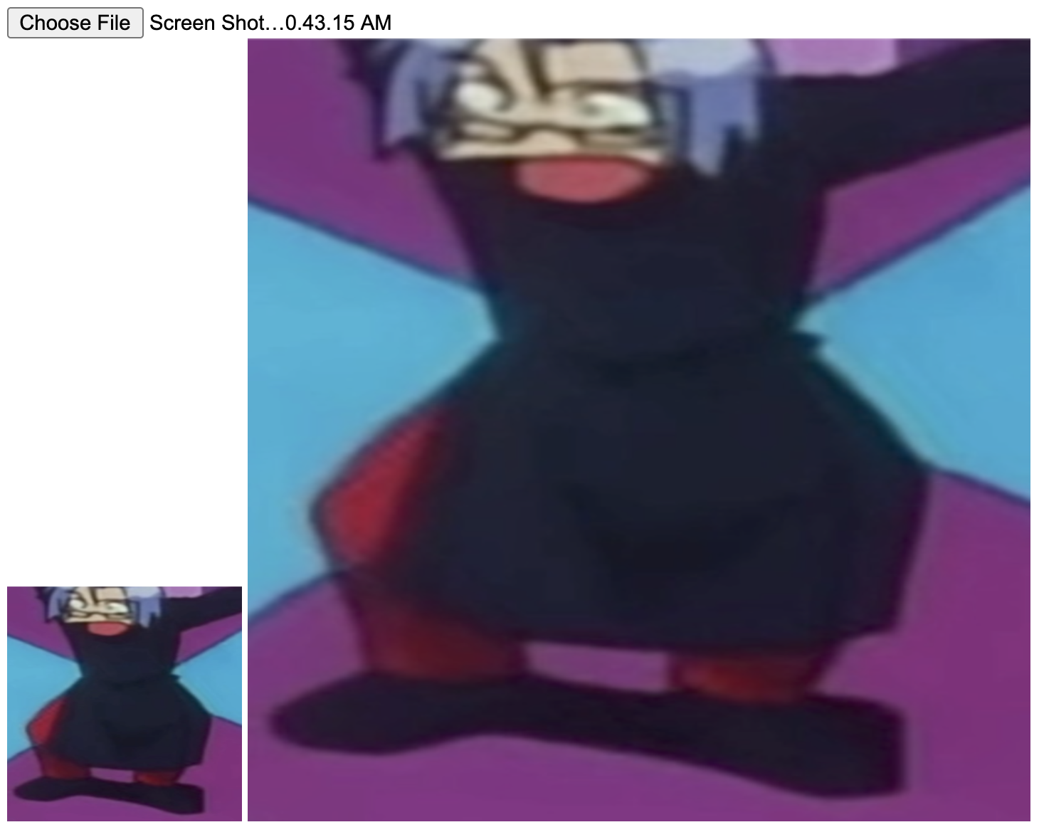
As I said, the main problem here is that Ash can't recognize Team Rocket. Want to see the evidence? Check this out:
Even though they wave big "R" flags, Ash is completely clueless. Wow. What about this one?
Yep, it's Team Rocket. Lastly,
So, Ash isn't the only one with the problem.
The object detection model
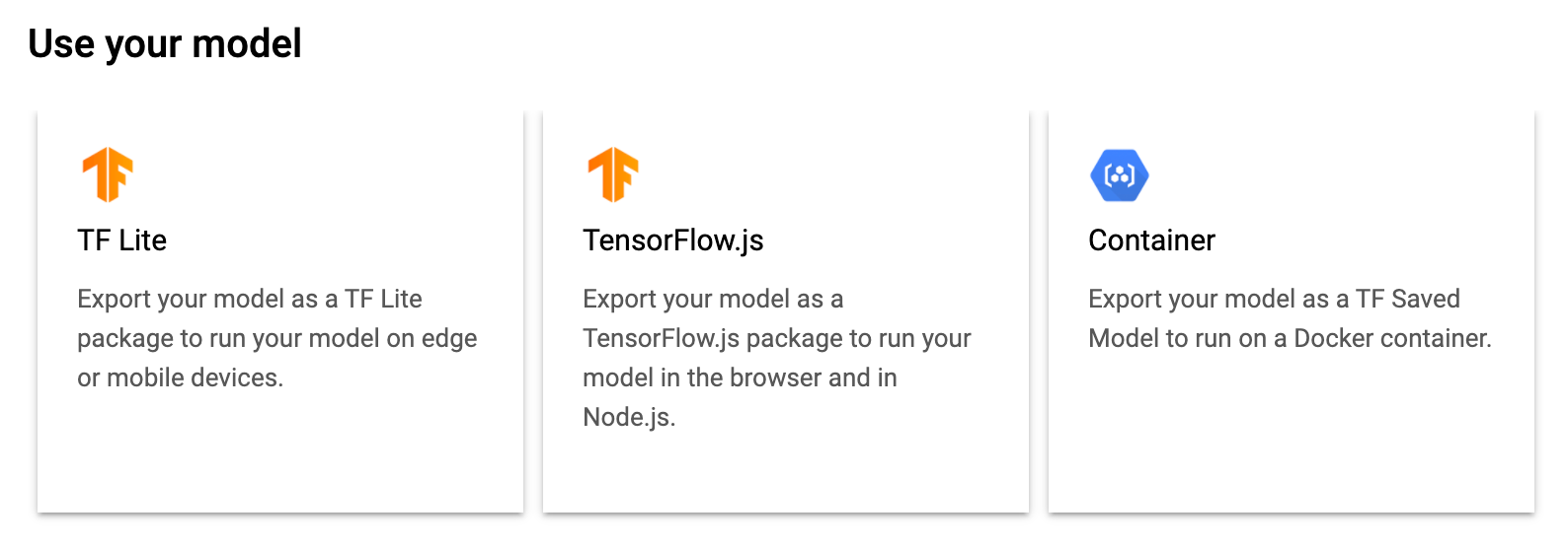
The first of the two models I created is an object detector trained using Google Cloud's AutoML Vision Object Detection. This service allows you to easily (and boringly) annotate an object detection dataset and train a model within a couple of clicks. The trained model can be exported and optimized for several inference engines such as TensorFlow.js, TensorFlow Lite, and TensorFlow.
The service is not free, though. However, Google provides a one-time credit voucher that should be enough for a small model.
Creating and annotating the dataset
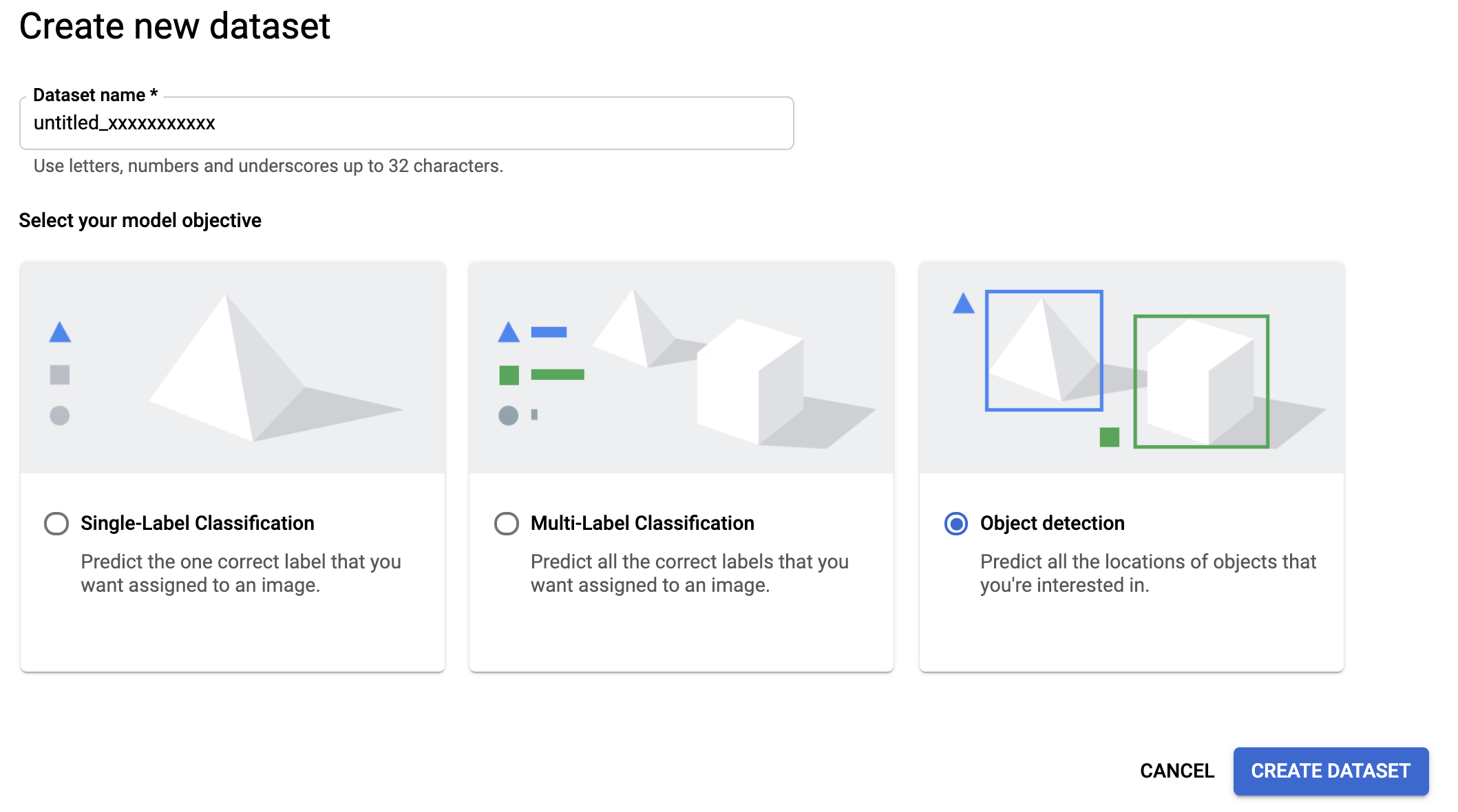
The first step needed before training an AutoML Object Detection model involves uploading the dataset and annotating it. To upload the data, access the dataset management page by searching for "dataset" in the Cloud Console search bar. Then, create a new dataset of type "object detection" (Figure 3) and upload the images to a bucket.
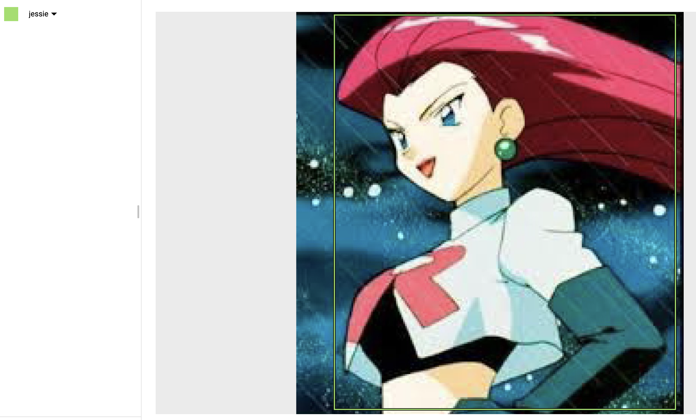
Once uploaded and processed, go to the "IMAGES" tab to start the dreary process of annotating the dataset. In this context, annotating a dataset consists of drawing the bounding boxes (Figure 4) of the target object(s) on top of the image—not that fun.
With the dataset labeled, click the "TRAIN" tab to train the model.
Training the model
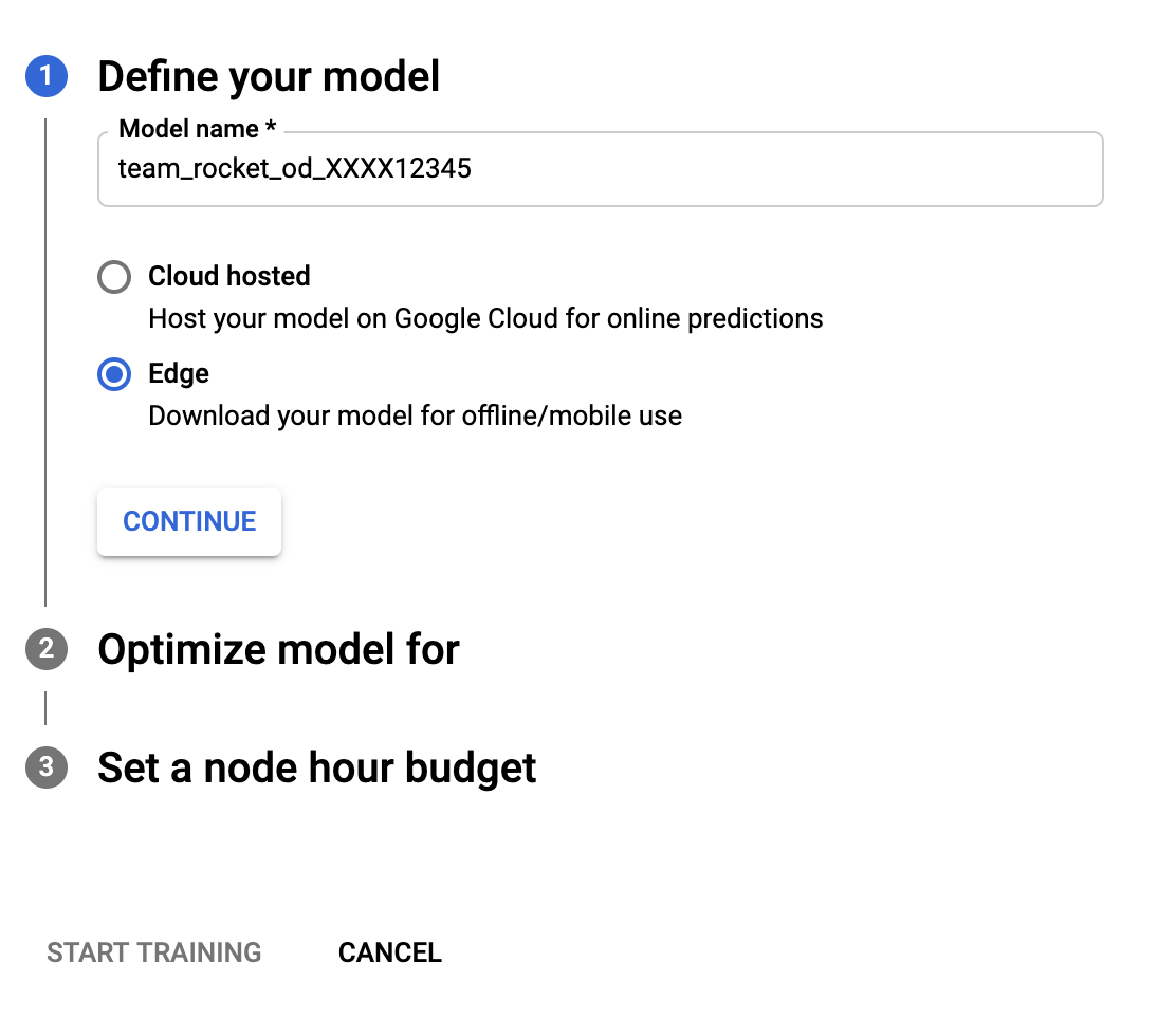
Training the model is done within three clicks. From the current screen, go to the "TRAIN" tab and click on "TRAIN NEW MODEL." Then, name the model, select "edge" (because we want to download it), choose the optimization target (I'm using higher accuracy), and the node hour budget, followed by clicking "START TRAINING." Using the default node hour budget, and with my dataset's size, the training took around 4 hours.
Evaluating the model
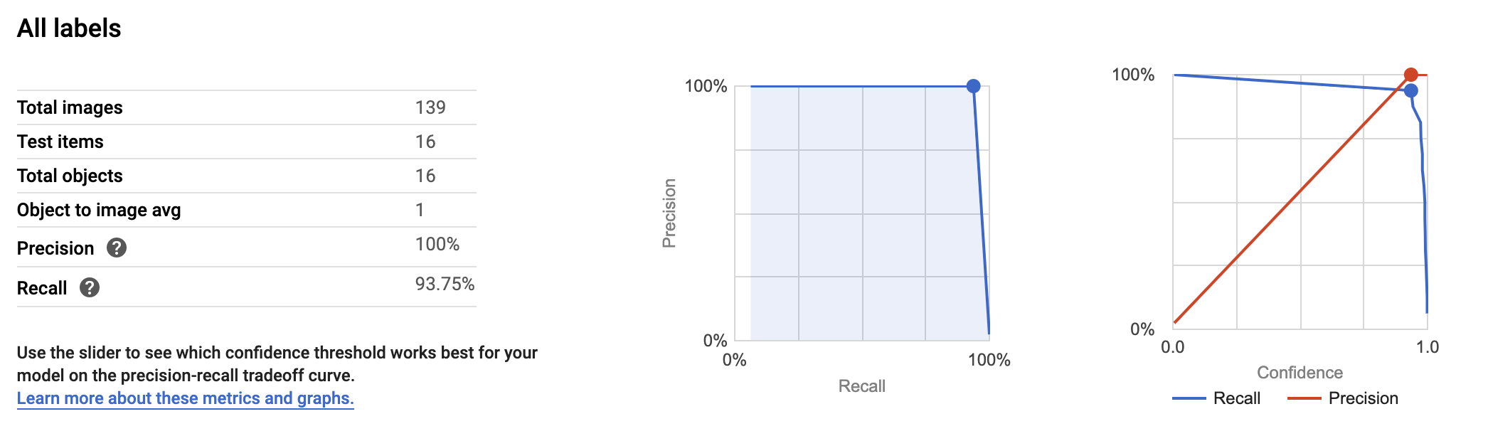
The training has ended; welcome back. To evaluate the model's metrics go to the "EVALUATE" tab. There you will find the precision and recall score and the option to calculate them at different threshold levels. My model achieved precision and recall of 100% and 93.75%, respectively (Figure 6). However, in practice, as we will soon see, the model is a bit worse. But that's ok! Considering the size of the training set, I wouldn't expect the model to be that great.
As for the last step, go to the "TEST & USE" tab to export the TensorFlow.js model (Figure 7). The exported directory should have a model.json (the model topology) and dict.txt files (the labels), and several .bin files (the weights). Now, let's build an app around the model.
Deploying the model in TensorFlow.js
To detect Team Rocket using the object detection model and to run the image classification model to present the activation maps, I built a web app that uses TensorFlow.js to load the models and predict with them. In this part, I'll show how I loaded the object detection model, predicted with it, and drew the bounding boxes. Let's start with the HTML:
<html>

<head>
    <script src="https://cdn.jsdelivr.net/npm/@tensorflow/tfjs"></script>
    <script src="https://cdn.jsdelivr.net/npm/@tensorflow/tfjs-automl"></script>
</head>

<body>
    <input id='input-image' type='file' accept='image/*'><br>
    <img id='output' style="height:150px; width:150px;">
    <canvas id="output-detection-canvas"></canvas>
    <div style="display:none;">
        <img id="output-detections" width="500" height="500">
    </div>
    <script src="index.js" type="module"></script>
</body>

</html>
In the head tags, I'm loading TensorFlow.js and AutoML Edge API, a package that loads and runs models produced with AutoML Edge. In the body, there is an input element used by the user to upload an image and two image tags. One displays the original image, and the second one, the image with the bounding boxes. Then, we call the JS script:
let odModel;
const odModelOptions = {
  score: 0.80,
  iou: 0.80,
  topk: 5,
};

let ctx;
const ODSIZE = 500;
const BBCOLOR = '#008000';


function setupODCanvas() {
  const canvas = document.getElementById('output-detection-canvas');
  ctx = canvas.getContext('2d');
  canvas.width = ODSIZE;
  canvas.height = ODSIZE;
}

function drawBoundingBoxes(prediction) {
  ctx.font = '20px Arial';
  const {
    left, top, width, height,
  } = prediction.box;

  // Draw the box.
  ctx.strokeStyle = BBCOLOR;
  ctx.lineWidth = 1;
  ctx.strokeRect(left, top, width, height);

  // Draw the label background.
  ctx.fillStyle = BBCOLOR;
  const textWidth = ctx.measureText(prediction.label).width;
  const textHeight = parseInt(ctx.font);

  // Top left rectangle.
  ctx.fillRect(left, top, textWidth + textHeight, textHeight * 2);
  // Bottom left rectangle.
  ctx.fillRect(left, top + height - textHeight * 2, textWidth + textHeight, textHeight * 2);

  // Draw labels and score.
  ctx.fillStyle = '#000000';
  ctx.fillText(prediction.label, left + 10, top + textHeight);
  ctx.fillText(prediction.score.toFixed(2), left + 10, top + height - textHeight);
}

function processInput() {
  const inputImage = document.getElementById('input-image');
  const outputDetections = document.getElementById('output-detections');

  // Fired when the user selects an image.
  inputImage.onchange = async (file) => {
    const input = file.target;
    const reader = new FileReader();
    const output = document.getElementById('output');

    // Fired when the selected image is loaded.
    reader.onload = () => {
      const dataURL = reader.result;

      // Set the the image to the output img element
      output.src = dataURL;
      // Set the the image to the canvas element
      outputDetections.src = dataURL;
    };

    // Fired when the image is loaded to the HTML.
    output.onload = async () => {
      const obPredictions = await odModel.detect(outputDetections, odModelOptions);
      ctx.drawImage(output, 0, 0, ODSIZE, ODSIZE);
      obPredictions.forEach((obPrediction) => {
        drawBoundingBoxes(obPrediction);
      });
    };

    reader.readAsDataURL(input.files[0]);
  };
}

async function init() {
  odModel = await tf.automl.loadObjectDetection('models/object-detection/model.json');
  setupODCanvas();
  processInput();
}

init();
At the top of the script, we declare the model variable and its options. The options object specifies the threshold, Intersect over Union (IoU) threshold, and the max number of objects to return. Following it is the context of the canvas where we'll draw the detections, the size of the output image, and the color the detection overlay.
The first function setupODCanvas() sets up the object detection canvas. The second one, drawBoundingBoxes(), is responsible for drawing the bounding boxes. Then, comes processInput(), the function that predicts. Here, we are using the onchange event of the image input element, to predict when the user selects an image. Once triggered, we get the image and use it as an argument to odModel.detect(), the method that detects the objects. After detecting, we draw the image and the bounding boxes on the canvas.
To run the web app, start a local web server in the project's root directory. You can easily create one using $ python3 -m http.server or with http-server, a command line tool for creating http servers. After starting the server, go to the address shown by the server, e.g., http://127.0.0.1:8080/, to access the app. Note that in the code I'm using the port 8080.
Is the model capable of detecting Team Rocket?
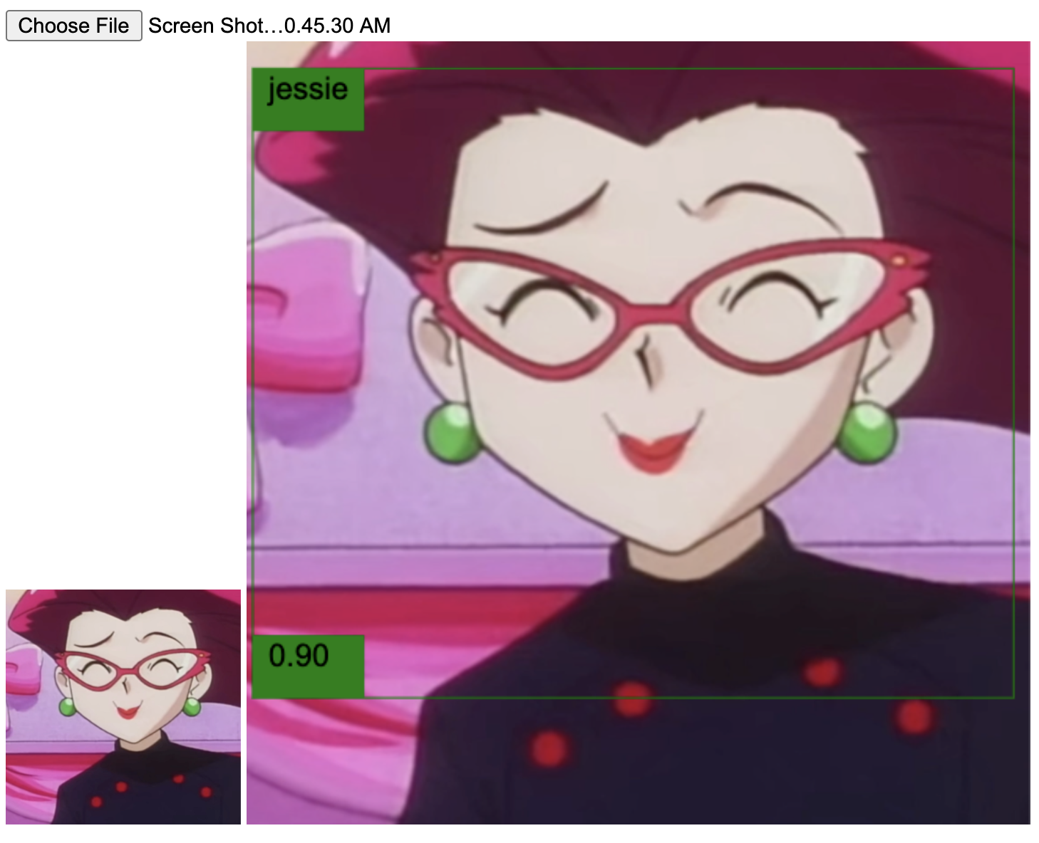
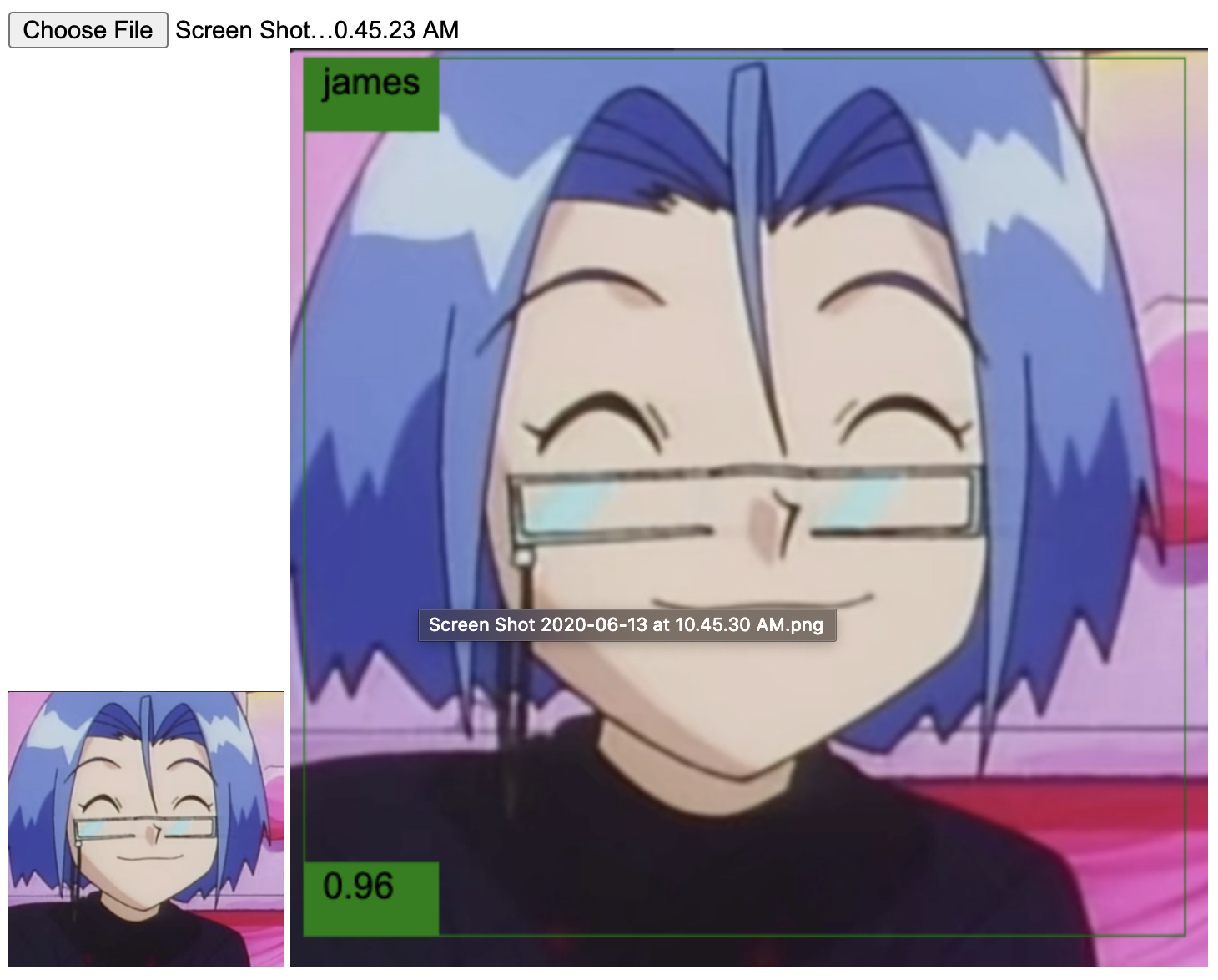
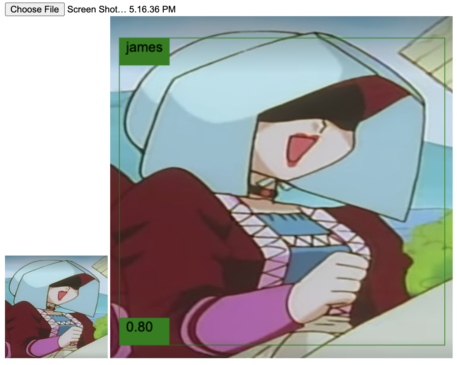
Empirically speaking, yes! It is capable of detecting Team Rocket better than Ash. But, like Ash, it also fails every now and then. Let's see. Below are some detections from scenes of the clips presented above.
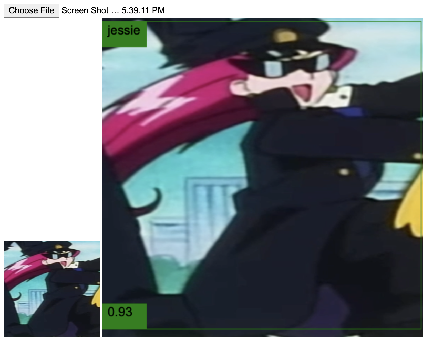
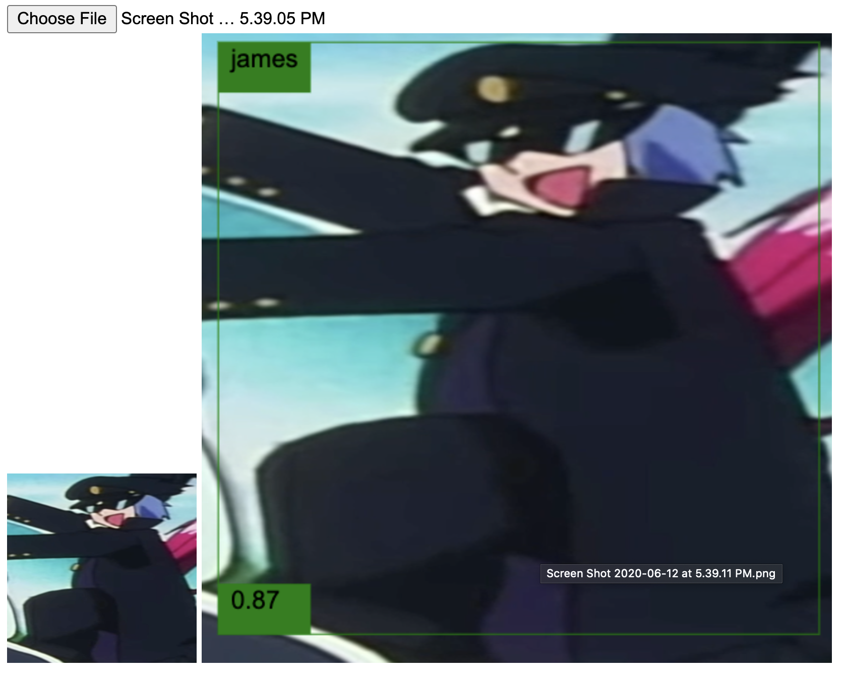
Good job, neural network! Those are indeed Jessie and James. The following ones are from the second video.
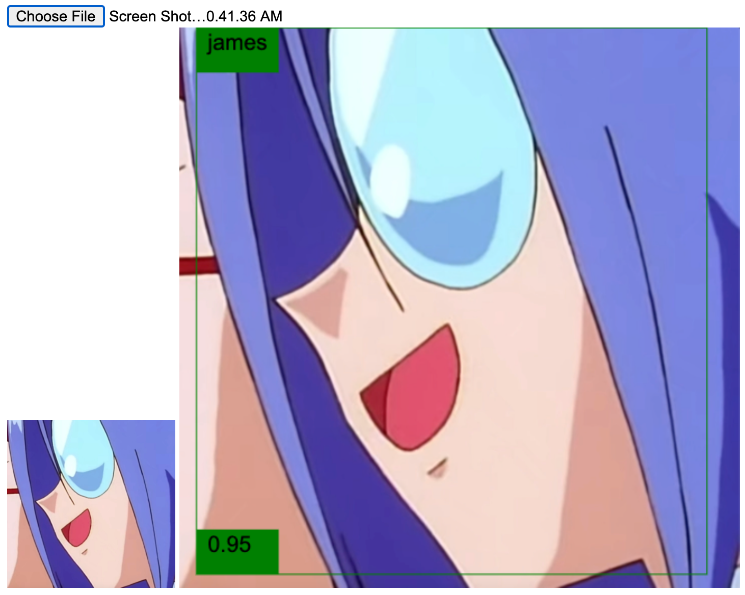
Again, success.
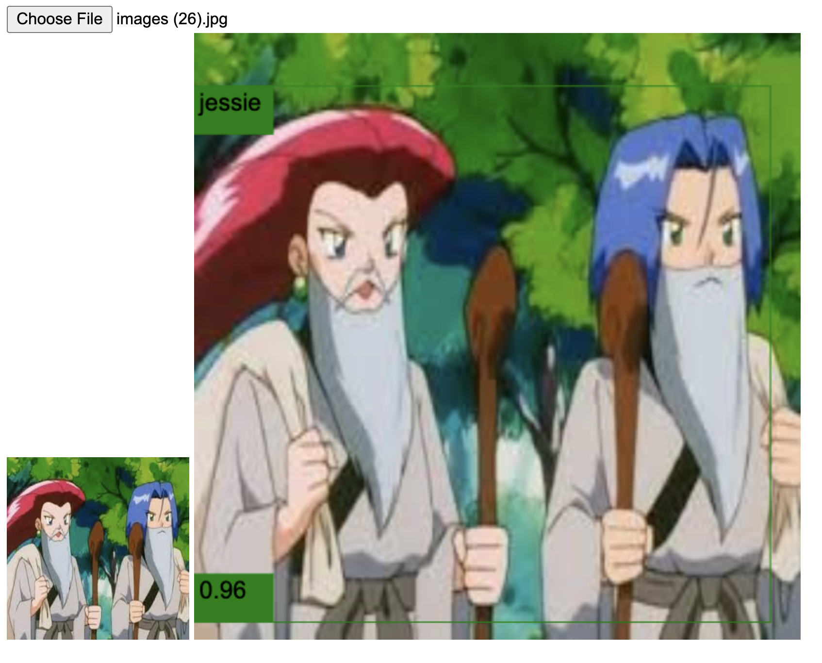
These were some of the positive cases where the model worked as planned. But unfortunately, there were others where it failed. I noticed that the model didn't perform well (at least with the same confidence threshold used in the others) in situations where Team Rocket looks too goofy, the images lack details, and where they are seen from far. For example:
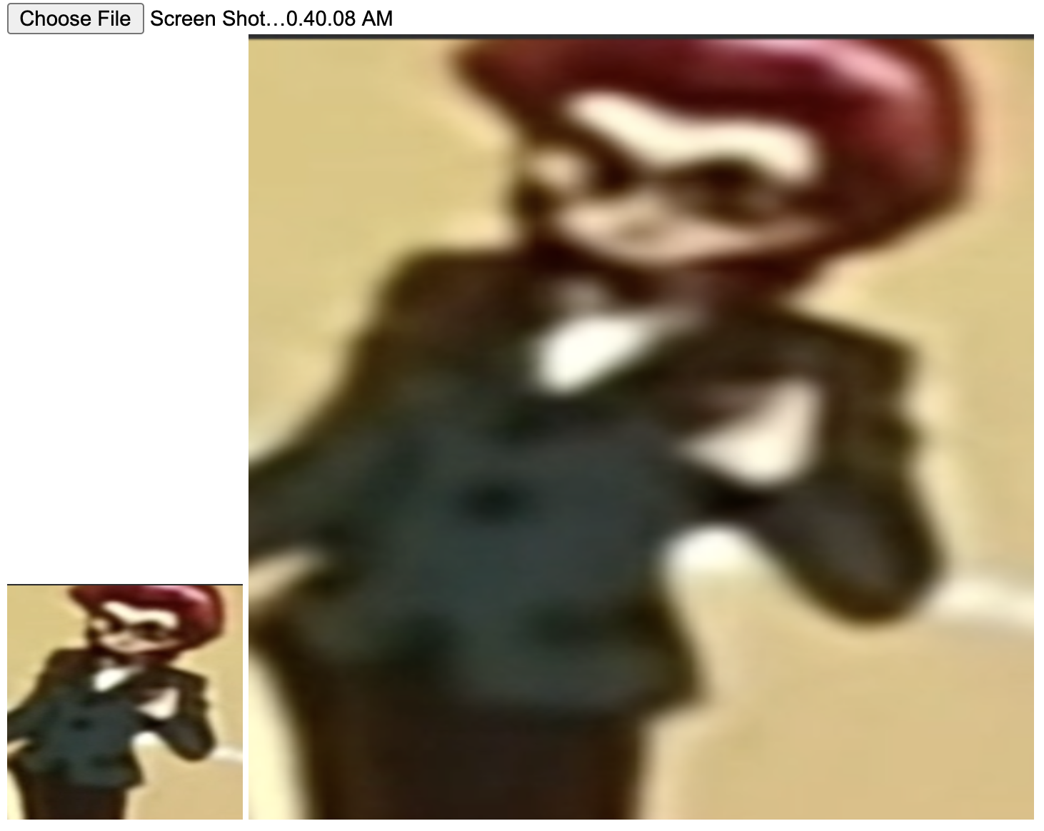
The network has issues detecting them in images that do not display their most distinguishable feature: the hair color. For example,
In the image above, you barely see Jessie's hair. Honestly, if I wouldn't know the context, I couldn't tell either that's her. Similarly, are cases where they dyed their hair:
The last of the issues I want to mention is that in none of my tests, the network was able to detect both members in one picture. Instead, it detects both of them as one label. This inconvenience, alongside the false positives, is, in my opinion, the biggest flaw of the experiment. I hope to fix it after adding more training data.
So, to summarize, is a neural network better than Ash at detecting Team Rocket? I say, yes. Now comes a follow-up question. How is the network identifying them? What does it see before saying, "yes, this is Jessie." In the second part of the experiment, I'm addressing this.
Interpreting the activation maps
In layman's terms, a convolutional neural network (CNN) learns to discern a category by looking at its most prominent visual features. For example, a CNN might learn that a banana is a banana because of its banana-ish shape and yellow color. For the second part of the experiment, I wanted to study the visual features a CNN extracts from an image of Jessie and James. In other words, I'm interested to see the network's activation maps, which are the outputs of its convolutional and max pooling layers.
To achieve this goal, I trained in TensorFlow, a CNN image classifier that predicts if an image is of Jessie or James. That way, I'll know why the network believes this is either Jessie or James. With the network trained, I expanded the previous TensorFlow.js app to load the model and plot on screen the activation maps of all the layers and each filter. It looks like this:
Training the model
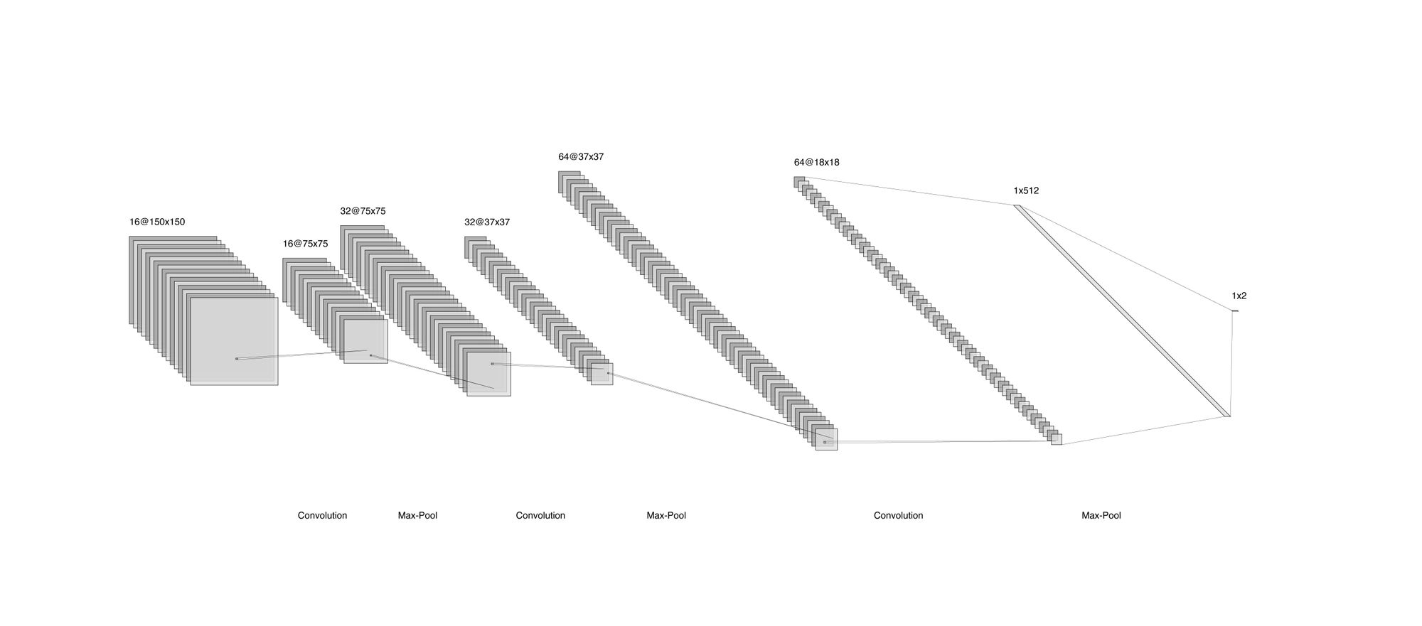
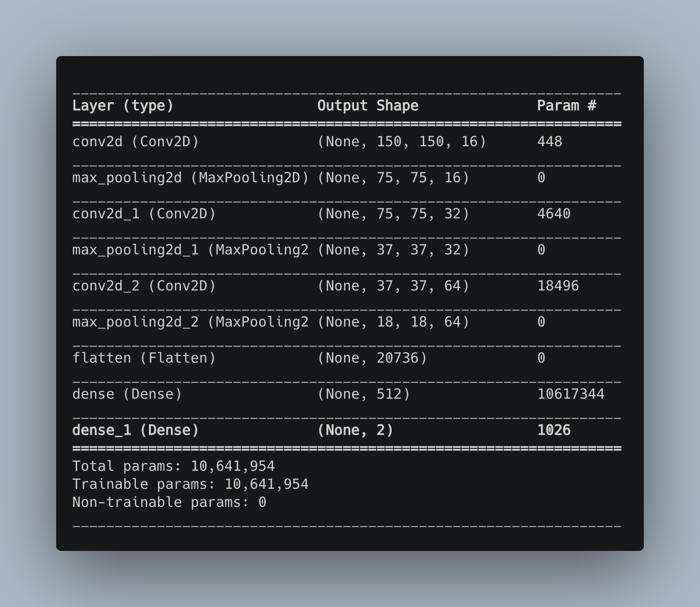
The image classifier model is a pretty standard CNN. It has three convolutional layers, three max pooling layers, one dropout layer, a dense layer with the ReLU activation function, and as for the last one, another dense of two units and softmax activation function. This last bit means that the output is a vector of length 2, where each value is the likelihood of the image being of James (label 0) or Jessie (label 1). Below is a diagram of the model, followed by its summary.
Unlike the previous model, for training this one, I have a richer dataset. Well kind of. Instead of using the 158 images, I'm using TensorFlow's Image Generator to augment my dataset by transforming the existing dataset. The transformations I'm applying rotate the image between [-45, 45] degree, shifts it horizontally and vertically, flips it horizontally, and zooms it. Moreover, 20% of the generated images are used as the validation set. To evaluate the model, I'm using TensorBoard. Below is the complete training script:
import datetime

import matplotlib.pyplot as plt
import tensorflow as tf
from tensorflow.keras.layers import Conv2D, Dense, Flatten, MaxPooling2D
from tensorflow.keras.models import Sequential
from tensorflow.keras.preprocessing.image import ImageDataGenerator

BATCH_SIZE = 64
EPOCHS = 25
IMG_HEIGHT = 150
IMG_WIDTH = 150


def create_data_generators():
    """Create the data generators used for training.

    Returns:
        tf.keras.preprocessing.image.ImageDataGenerator: Two ImageDataGenerator;
        the training and validation dataset.
    """
    image_gen_train = ImageDataGenerator(
        rescale=1./255,
        rotation_range=45,
        width_shift_range=.15,
        height_shift_range=.15,
        horizontal_flip=True,
        zoom_range=0.2,
        validation_split=0.2
    )

    # James is label 0
    train_data_gen = image_gen_train.flow_from_directory(batch_size=BATCH_SIZE,
                                                         directory='data/train/',
                                                         shuffle=True,
                                                         target_size=(
                                                             IMG_HEIGHT, IMG_WIDTH),
                                                         class_mode='categorical',
                                                         subset='training')

    val_data_gen = image_gen_train.flow_from_directory(batch_size=BATCH_SIZE,
                                                       directory='data/train/',
                                                       shuffle=True,
                                                       target_size=(
                                                           IMG_HEIGHT, IMG_WIDTH),
                                                       class_mode='categorical',
                                                       subset='validation')

    return train_data_gen, val_data_gen


def train(train_data_gen, val_data_gen):
    # Set up TensorBoard directory and callback
    ts = datetime.datetime.now().strftime("%Y%m%d-%H%M%S")
    log_dir = "/tmp/tensorboard/{}".format(ts)
    tensorboard_callback = tf.keras.callbacks.TensorBoard(
        log_dir=log_dir, histogram_freq=1)

    model = Sequential([
        Conv2D(16, 3, padding='same', activation='relu',
               input_shape=(IMG_HEIGHT, IMG_WIDTH, 3)),
        MaxPooling2D(),
        Conv2D(32, 3, padding='same', activation='relu'),
        MaxPooling2D(),
        Conv2D(64, 3, padding='same', activation='relu'),
        MaxPooling2D(),
        Flatten(),
        Dense(512, activation='relu'),
        Dense(2, activation='softmax')
    ])

    model.compile(optimizer='adam',
                  loss=tf.keras.losses.CategoricalCrossentropy(),
                  metrics=['accuracy'])

    model.fit(
        train_data_gen,
        steps_per_epoch=train_data_gen.samples // BATCH_SIZE,
        epochs=EPOCHS,
        validation_data=val_data_gen,
        callbacks=[tensorboard_callback]
    )

    print(model.summary())
    model.save('models/{}'.format(ts))


if __name__ == "__main__":
    train_data_gen, val_data_gen = create_data_generators()
    train(train_data_gen, val_data_gen)
The first function create_data_generators() creates the generators (of course it does that, hahaha). train(), whose parameters are both generators, trains the model. Note that we are using the TensorBoard callback on model.fit() to log the model's training information. Once the training finishes, we save the model.
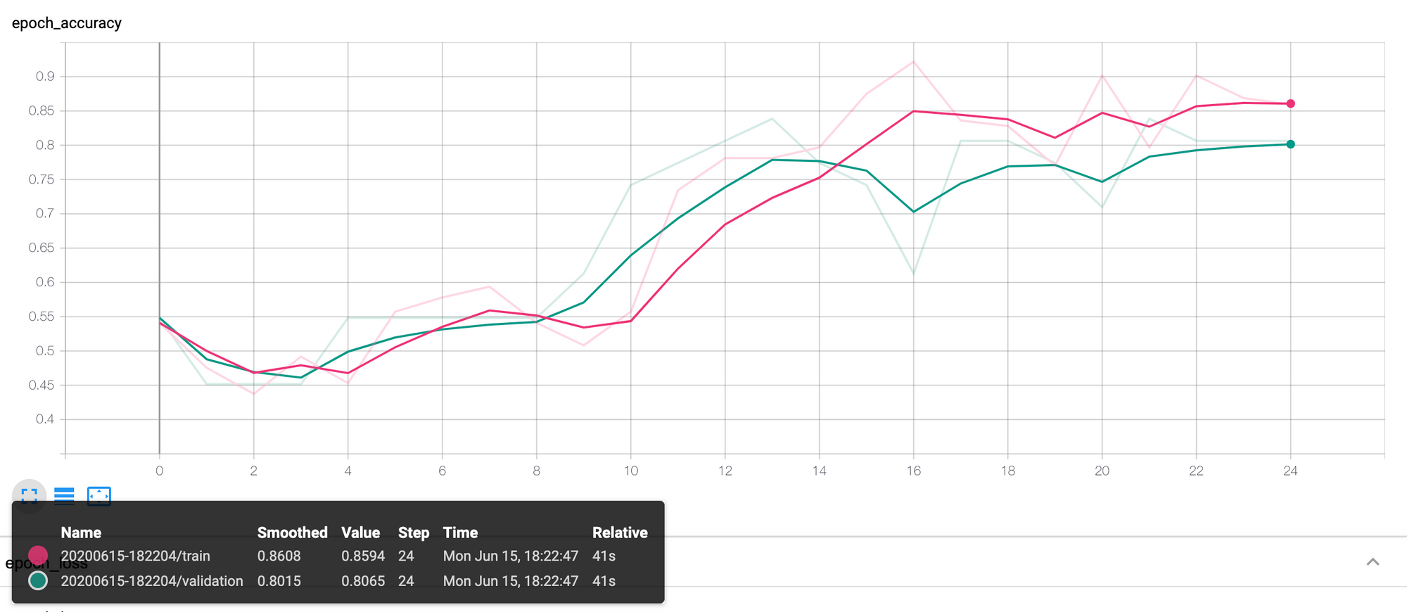
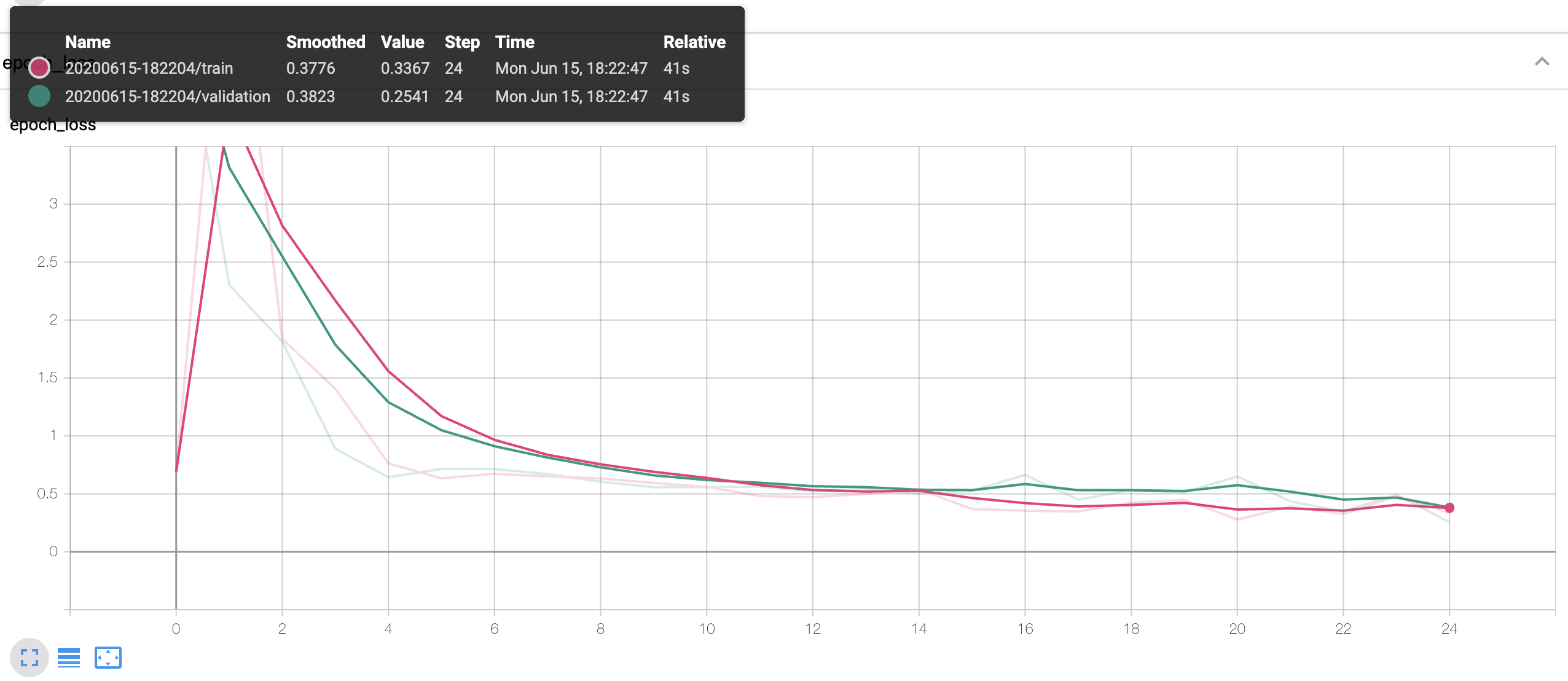
Regarding the model's performance, after 25 epochs, it achieved a training accuracy and loss value of 0.8594 and 0.3367, respectively, and validation accuracy and loss value of 0.8065 and 0.2541. Below are two screenshots from TensorBoard presenting the accuracy and loss values.
To launch TensorBoard, execute in the terminal:
$ tensorboard --logdir /tmp/tensorboardMake sure the given path is the same one used in the TensorBoard callback used in model.fit().
Converting the model to a TensorFlow.js model
At the end of the training, we save the model to disk. However, this format won't work in TensorFlow.js. To use the model in our web app, we must first convert it to TensorFlow.js format; it is easier than it sounds. To convert it, we need the TensorFlow.js Converter tool. After installing it, execute the following command to produce the TensorFlow.js version of the model:
$ tensorflowjs_converter --input_format=keras_saved_model PATH/TO/TS_MODEL OUTPUT/PATHThe TensorFlow.js activation web app
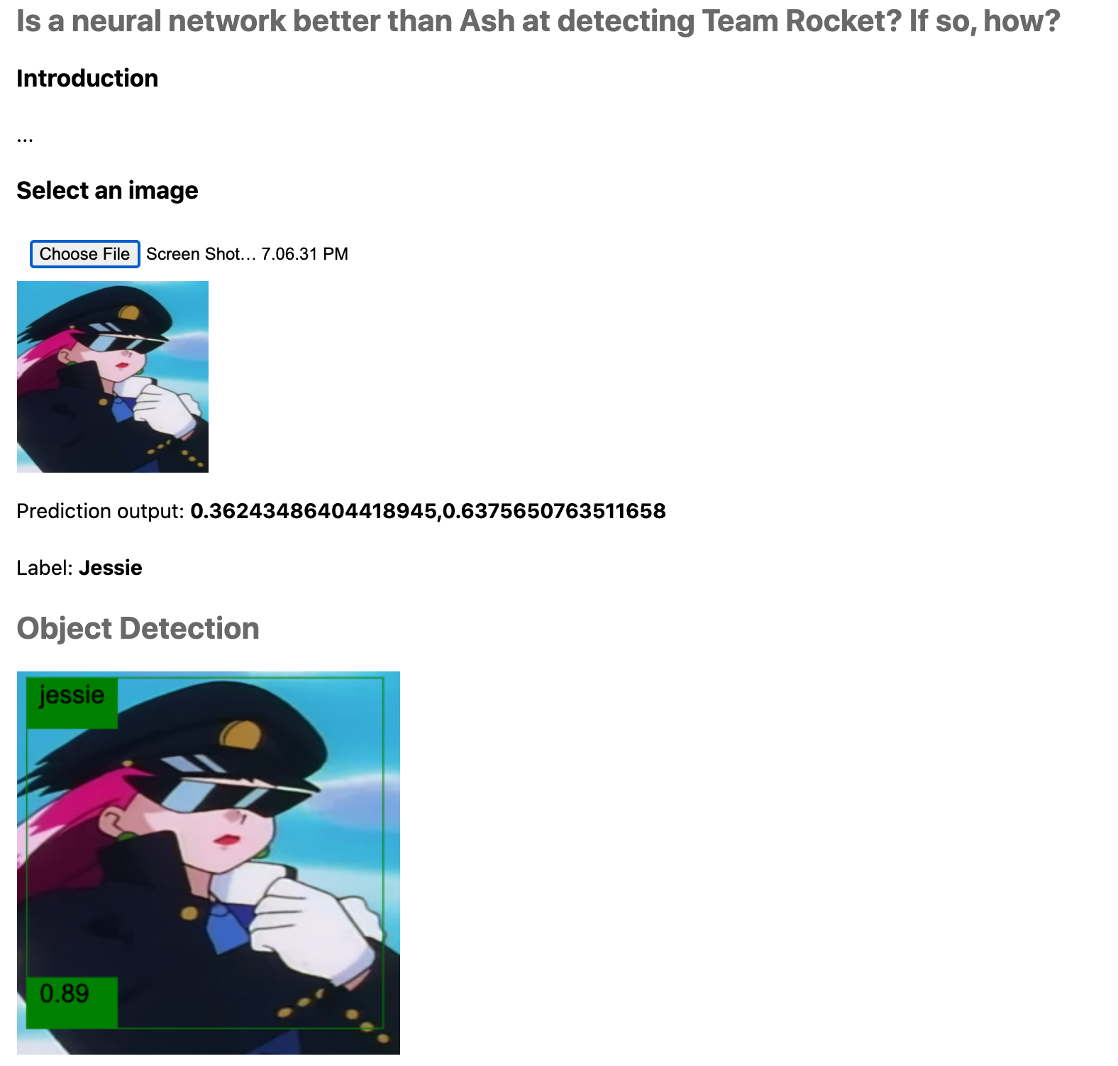
The activation map web app we will see here is an extension of the previous one. Now, besides detecting Team Rocket, it will classify the image between "Jessie" or "James" and present the layer's activation maps.
You can find the app at https://juandes.github.io/team-rocket-activations-app/index.html.
Figure 20 is a screenshot of the app. There you can see the image input control, the object detection canvas, the prediction outcome, and one section per layer, where the user uses an input slider to select the filter it wants to visualize. How did I build the app? Time for some code, starting with the HTML:
<html>

<head>
    <script src="https://cdn.jsdelivr.net/npm/@tensorflow/tfjs"></script>
    <script src="https://cdn.jsdelivr.net/npm/@tensorflow/tfjs-automl"></script>
    <script src='https://cdn.plot.ly/plotly-latest.min.js'></script>
    <link href="./style.css" rel="stylesheet">
</head>

<body>
    <div class="main-centered-container">
        <h2>Is a neural network better than Ash at detecting Team Rocket? If so, how?</h2>
        <h3>Introduction</h3>
        <p>...</p>
        <h3>Select an image</h3>
        <input id='input-image' type='file' accept='image/*'><br>
        <img id='output-image' style="height:150px; width:150px;">


        <p>Prediction output: <span id="p-prediction" style="font-weight:bold"></span></p>
        <p>Label: <span id="p-label" style="font-weight:bold"></span></p>
        <h2>Object Detection</h2>
        <canvas id="output-detection-canvas"></canvas>
        <div style="display:none;">
            <img id="output-detections" width="300" height="300">
        </div>

        <h2>Activations Maps</h2>
        <div id="activations-layer-one">
            <h3>conv2d layer activations</h3>
            <div>
                <input type="range" min="0" max="15" value="0" id="activations-layer-one-range">
                <p>Filter number: <span id="activations-layer-one-value"></span></p>
            </div>
            <div id="plot-activations-one"></div>
        </div>
        <div id="activations-layer-two">
            <h3>max_pooling2d activations</h3>
            <div>
                <input type="range" min="0" max="15" value="0" id="activations-layer-two-range">
                <p>Filter number: <span id="activations-layer-two-value"></span></p>
            </div>
            <div id="plot-activations-two"></div>
        </div>
        <div id="activations-layer-three">
            <h3>conv2d_1 activations</h3>
            <div>
                <input type="range" min="0" max="31" value="0" id="activations-layer-three-range">
                <p>Filter number: <span id="activations-layer-three-value"></span></p>
            </div>
            <div id="plot-activations-three"></div>
        </div>
        <div id="activations-layer-four">
            <h3>max_pooling2d_1 activations</h3>
            <div>
                <input type="range" min="0" max="31" value="0" id="activations-layer-four-range">
                <p>Filter number: <span id="activations-layer-four-value"></span></p>
            </div>
            <div id="plot-activations-four"></div>
        </div>
        <div id="activations-layer-five">
            <h3>conv2d_2 activations</h3>
            <div>
                <input type="range" min="0" max="63" value="0" id="activations-layer-five-range">
                <p>Filter number: <span id="activations-layer-five-value"></span></p>
            </div>
            <div id="plot-activations-five"></div>
        </div>
        <div id="activations-layer-six">
            <h3>max_pooling2d_2 activations</h3>
            <div>
                <input type="range" min="0" max="63" value="0" id="activations-layer-six-range">
                <p>Filter number: <span id="activations-layer-six-value"></span></p>
            </div>
            <div id="plot-activations-six"></div>
        </div>
        <script src="index.js" type="module"></script>
    </div>
</body>

</html>
For this version of the app, I'm using the visualization library Plotly to visualize the activation maps. Also, there is a CSS file you can find in the repo. In the body, there are two <p> 's that show the prediction label and output and six <div>'s (one per layer) with an input of type range used to select the filter we wish to plot—the max value is the number of filters the layer has. Each of these <div>'s have another <div> where the script programmatically adds the Plotly graph.
That’s the HTML. As for the JS script, before jumping into the code, let me quickly explain how it works. The script uses three models, the object detector, the image classifier, and a new model. This new model outputs a tensor made of all the intermediate activation maps. We will create this model by explicitly setting its input to the input of the image classifier and as output a list of the classifier’s output tensors (the convolutional and pooling layers). To trigger the predictions, the user first has to upload an image. After that, we will present the detected Rocket, the classification output, and the activation maps on the app. Now, let’s see the code part by part:
// The image classifier
let classifierModel;

// The image classifier used for creating the activation maps
let activationModel;

// The object detection model
let odModel;
const odModelOptions = {
  score: 0.80,
  iou: 0.80,
  topk: 5,
};


let imageTensor;
let ctx;

const BBCOLOR = '#008000';
const ODSIZE = 300;

const layersInformation = [
  {
    layer: 'one',
    size: 150,
  },
  {
    layer: 'two',
    size: 75,
  },
  {
    layer: 'three',
    size: 75,
  },
  {
    layer: 'four',
    size: 37,
  },
  {
    layer: 'five',
    size: 37,
  },
  {
    layer: 'six',
    size: 18,
  },
];
Above we have the models' variables: the image classifier, the model we will use to get the activations, and the object detector. Following them is the variable that holds the image we want to classify, the canvas context, and a list of maps that describe some information about the layers.
The first two functions I want to present are setupODCanvas() (from before) and initSliders(), used for initializing the sliders' input. initSliders()'s second parameter is a callback that's called when the user moves the slider:
function setupODCanvas() {
  const canvas = document.getElementById('output-detection-canvas');
  ctx = canvas.getContext('2d');
  canvas.width = ODSIZE;
  canvas.height = ODSIZE;
}

function initSliders(layerNumber, onInputCb) {
  const slider = document.getElementById(`activations-layer-${layerNumber}-range`);
  const output = document.getElementById(`activations-layer-${layerNumber}-value`);
  output.innerHTML = slider.value;

  slider.oninput = function getSliderValue() {
    output.innerHTML = this.value;
    onInputCb(this.value);
  };
}
Then comes drawActivation(), the one that draws the activation maps in the Plotly plot. Its parameters are all the "predicted" activations, the index of the layer whose filter we want to draw, the filter index, the id of the plot's <div>, and the size of the filter. Inside the function, we use tf.tidy(fn), a TensorFlow.js function that cleans up all the intermediate tensors allocated by fn. In tf.tidy(), we get the activation tensor and filter indicated by layerIndex and filterNumber. Then, we transform the activation map into a 2D array and plot it as a heatmap:
async function drawActivation(activations, layerIndex, filterNumber, plotId, size) {
  // Use tf.tidy to remove garbage collect the intermediate tensors.
  const activationToDraw = tf.tidy(() => {
    // Get the activation map of the given layer (layerIndex) and filter (filterNumber).
    const activation = activations[layerIndex].slice([0, 0, 0, filterNumber], [1, size, size, 1]);

    // TypedArray to Array and reverse it on the axis #1.
    const activationArray = Array.from(activation.reverse(1).dataSync());

    const reshapedActivation = [];
    // Reshape array to 2D
    while (activationArray.length) reshapedActivation.push(activationArray.splice(0, size));
    return reshapedActivation;
  });

  const data = [
    {
      z: activationToDraw,
      type: 'heatmap',
    },
  ];

  const layout = {
    autosize: false,
    width: 500,
    height: 500,
  };

  Plotly.newPlot(plotId, data, layout);
}
After it is setupSliders(). This one iterates over layersInformation and calls initSliders() using the values from layersInformation. The second parameter of initSliders() is the callback that triggers when the person uses the slider to select a filter of the layer. In that event, we will produce the activations maps using activationModel. After prediction, we call drawActivation():
function setupSliders() {
  layersInformation.forEach((layerInfo, i) => {
    initSliders(layerInfo.layer, (filterNumber) => {
      const activations = activationModel.predict(imageTensor);
      drawActivation(activations, i, parseInt(filterNumber), `plot-activations-${layerInfo.layer}`, layerInfo.size);
    });
  });
}
Next is setupModels(), responsible for initializing the three models we're using. The function starts by loading the classifier and object detection models. After that, it iterates over the first six layers of the CNN (the three convolutional and max pooling) and adds their outputs to a list. We then create a new model named activationModel using TensorFlow's functional approach in which we have to specify the model's inputs and outputs:
async function setupModels() {
  classifierModel = await tf.loadLayersModel('models/tfjs-version/model.json');
  odModel = await tf.automl.loadObjectDetection('models/object-detection/model.json');

  const outputLayers = [];

  // Iterate over first six layers of the image classification model
  // and push their output to outputLayers
  classifierModel.layers.slice(0, 6).forEach((layer) => {
    outputLayers.push(layer.output);
  });


  activationModel = tf.model({ inputs: classifierModel.inputs, outputs: outputLayers });
  activationModel.summary();
}
The following function is the same drawBoundingBoxes() from before:
function drawBoundingBoxes(prediction) {
  ctx.font = '20px Arial';
  const {
    left, top, width, height,
  } = prediction.box;

  // Draw the box.
  ctx.strokeStyle = BBCOLOR;
  ctx.lineWidth = 1;
  ctx.strokeRect(left, top, width, height);

  // Draw the label background.
  ctx.fillStyle = BBCOLOR;
  const textWidth = ctx.measureText(prediction.label).width;
  const textHeight = parseInt(ctx.font);

  // Top left rectangle.
  ctx.fillRect(left, top, textWidth + textHeight, textHeight * 2);
  // Bottom left rectangle.
  ctx.fillRect(left, top + height - textHeight * 2, textWidth + textHeight, textHeight * 2);

  // Draw labels and score.
  ctx.fillStyle = '#000000';
  ctx.fillText(prediction.label, left + 10, top + textHeight);
  ctx.fillText(prediction.score.toFixed(2), left + 10, top + height - textHeight);
}
Now comes the first function that predicts. This one, named predictWithObjectDetector(), uses the input image to detect Team Rocket just like we did before:
async function predictWithObjectDetector(outputDetections, outputImage) {
  // Predict with the object detector.
  const obPredictions = await odModel.detect(outputDetections, odModelOptions);

  ctx.drawImage(outputImage, 0, 0, ODSIZE, ODSIZE);
  obPredictions.forEach((obPrediction) => {
    drawBoundingBoxes(obPrediction);
  });
}
The next function, named predictWithClassifier(), gets the input image, converts it to a tensor, and predicts its label, and activations. After predicting, the function draws the activation maps of the first filter from every layer and adds the prediction outcome to the HTML. This function runs when a user uploads an image. Unlike the prediction we did on the callback from initSliders(), where the drew the activations of the filter selected by the user, here we will visualize the first filter of each layer:
function predictWithClassifier(image) {
  // Convert the image to a tensor.
  imageTensor = tf.browser.fromPixels(image)
    .expandDims()
    .toFloat()
    .div(255.0);

  const prediction = classifierModel.predict(imageTensor).dataSync();
  const activations = activationModel.predict(imageTensor);

  // Draw the activation maps of the first filter.
  layersInformation.forEach((layerInfo, i) => {
    drawActivation(activations, i, 0, `plot-activations-${layerInfo.layer}`, layerInfo.size);
  });

  document.getElementById('p-prediction').innerHTML = prediction;
  // argMax returns a tensor with the arg max index. So,
  // we need dataSync to convert it to array and indexing to
  // get the value.
  const label = tf.argMax(prediction).dataSync()[0];

  document.getElementById('p-label').innerHTML = ((label === 0) ? 'James' : 'Jessie');
}
Then is the function that glues everything together: processInput(). This function uses several events to load the image selected by the user, draws it on screen, and call the previous predict functions:
function processInput() {
  const inputImage = document.getElementById('input-image');
  const outputDetections = document.getElementById('output-detections');

  // Fired when the user selects an image.
  inputImage.onchange = async (file) => {
    const input = file.target;
    const reader = new FileReader();
    const outputImage = document.getElementById('output-image');

    // Fired when the selected image is loaded.
    reader.onload = () => {
      const dataURL = reader.result;

      // Set the the image to the output img element
      outputImage.src = dataURL;
      // Set the the image to the canvas element
      outputDetections.src = dataURL;
    };

    // Fired when the image is loaded to the HTML.
    outputImage.onload = async () => {
      predictWithObjectDetector(outputDetections, outputImage);
      predictWithClassifier(outputImage);
    };

    reader.readAsDataURL(input.files[0]);
  };
}
Last, there’s an init function which serves as the app’s starting point.
async function init() {
  setupODCanvas();
  setupSliders();
  await setupModels();
  processInput();
}


init();
That's for the code. To run the app, follow the approach previously discussed.
How is the model identifying Team Rocket?
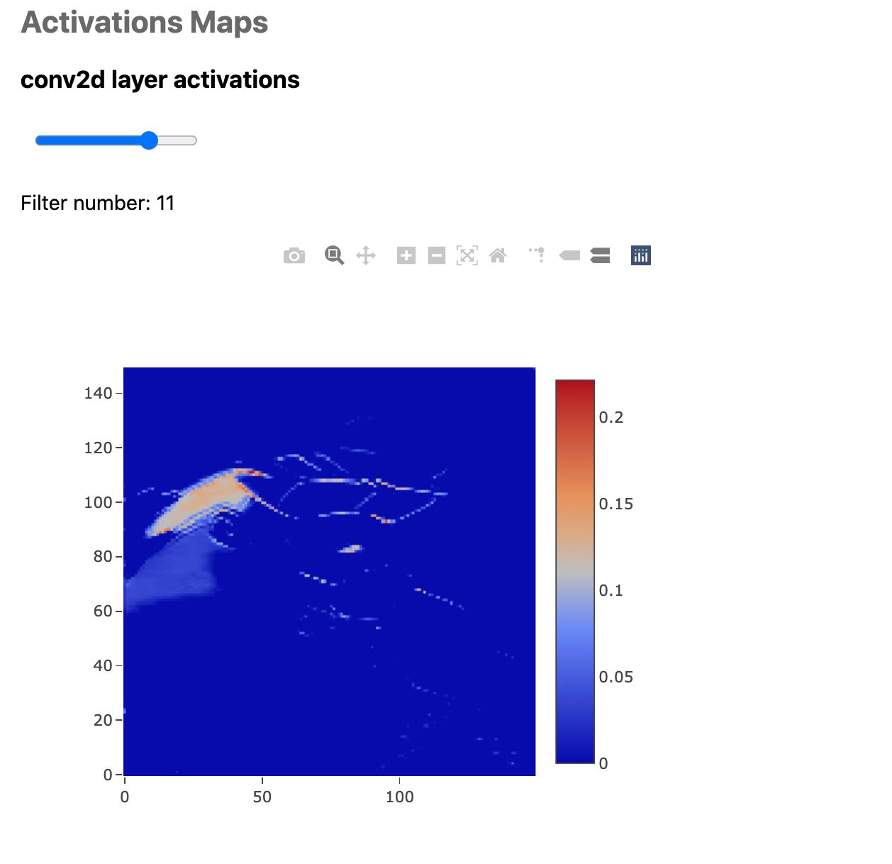
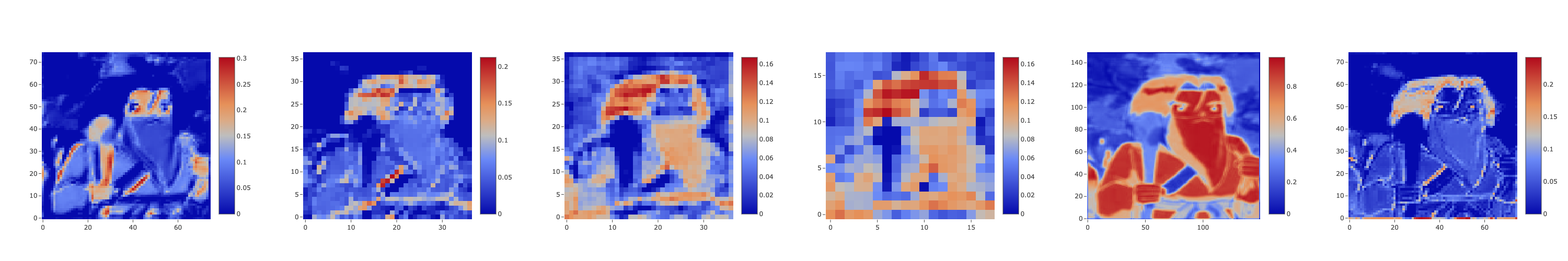
After that nice TensorFlow.js and JS lesson, it's time to answer our second question, how is the model identifying Team Rocket? What does it see at prediction time? To answer it, I'll present several activation maps, starting by those from created by following image:

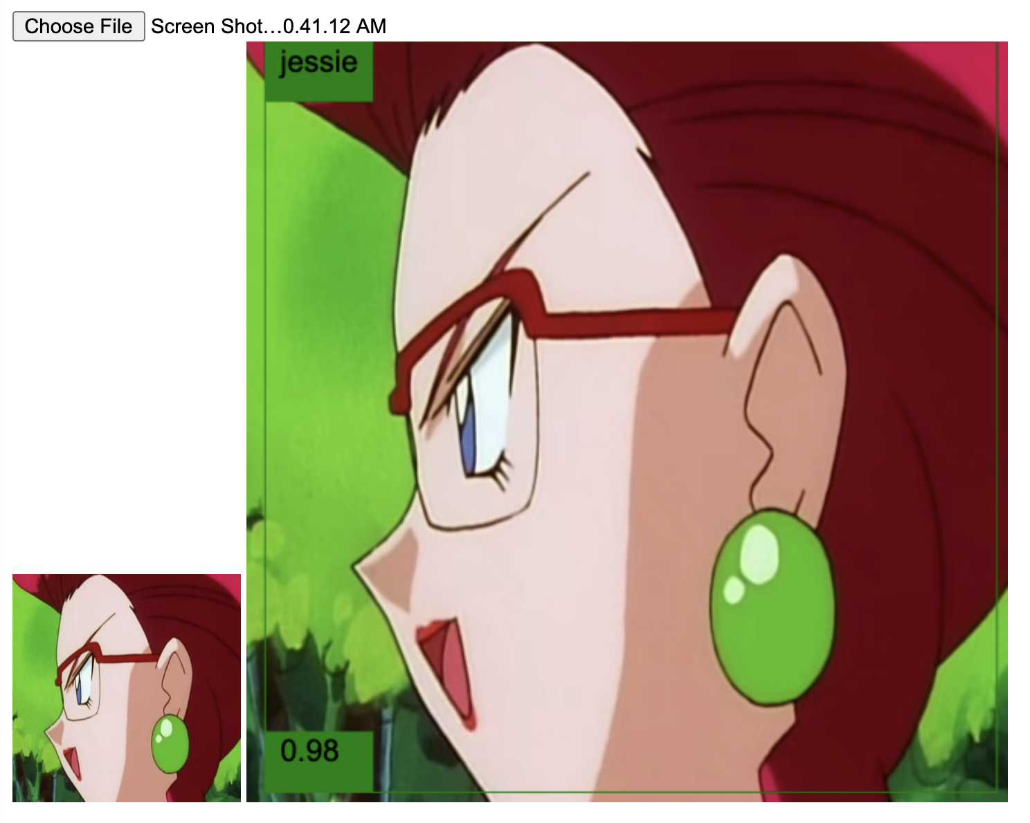
The CNN says this is Jessie—0.99 Jessie and 0.01 James, according to the softmax output. But why is it her? Well, see for yourself.
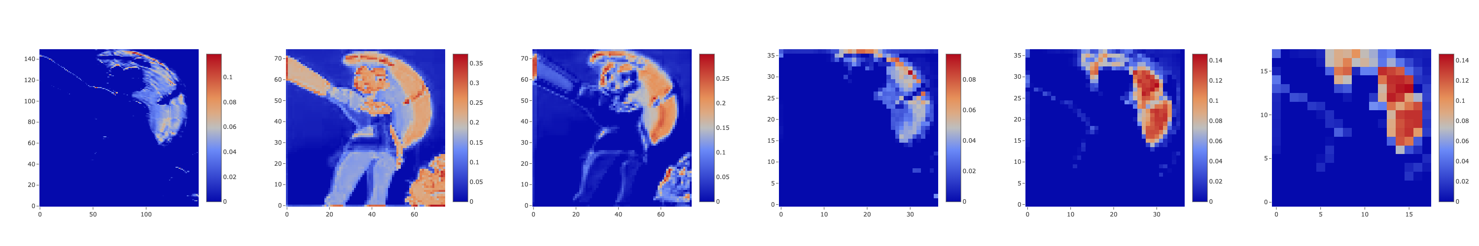
Figure 26 presents the activations maps of some filters from the six layers. The first two images come from the first convolutional and max pooling layers. The two that follow are from the second set of convolutional and max pooling, and the last two, from the third set—since each consecutive layer is smaller than the previous one, the resolution of the images decreases. On these heatmaps, the color's intensity represents the regions the CNN uses to identify the object. And that's why it is not surprising that Jessie's hair, arguably her most icon feature, stands out.
These images, though, do not tell the complete story of the network. They are just a small sample from the 100+ filters the model has. While most of the maps focus on the hair, others look at other parts:
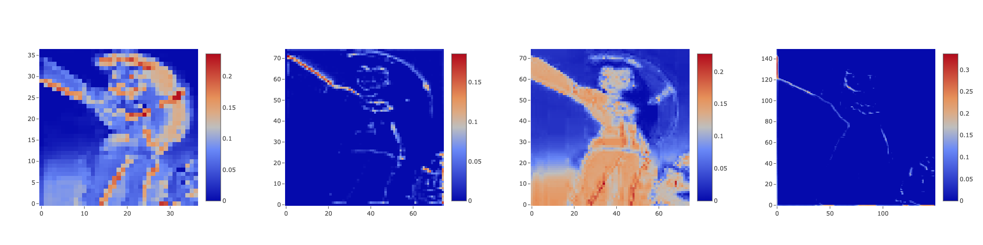
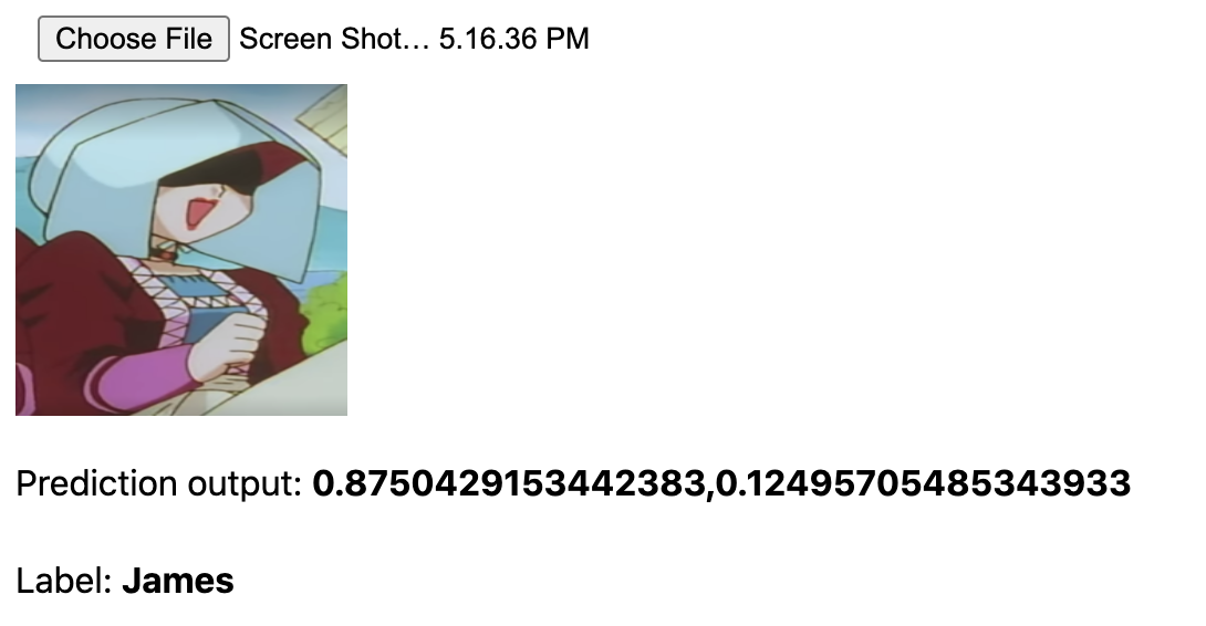
For the next example, consider this image of James:

The CNN correctly predicted "James" (Jessie 0.20, James 0.80). Like before the network is also mostly focusing on the hair, and in some cases, on that majestic fake beard.
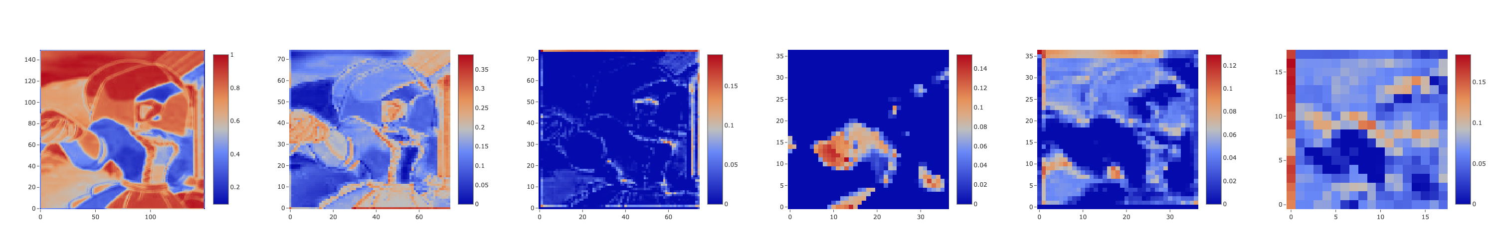
Nothing is perfect, and that includes my network. During my tests, I found some cases where the CNN prediction was wrong. One example is the same picture of Jessie that the object detector couldn't detect—we could say that's because the hair is hardly present.
Here are the activation maps. There's no distinguishable feature of Jessie being identified.
With that, we conclude the experiment! To see more examples, I'll invite you to check out the interactive demo presented above or to clone the repo and run it yourself.
Conclusion and recap
Life is full of questions. Who am I? Was it the chicken or the egg? Is a neural network better than Ash at detecting Team Rocket? In this experiment, I attempted to answer the latest. The results were satisfactory, and I'm willing to answer the question with a "yes." For the project, I trained two networks, an object detector and an image classifier to detect Team Rocket in an image and learn about the features a CNN sees as relevant. To use the models, we created a web app using TensorFlow.js that loads them and presents the detected Rocket and the activation maps.
To my dear friend Ash Ketchum, these are the tips I have for you. As we learned from the object detector model, if you are ever in the situation where you need to know if the group in front of you is Team Rocket, try to analyze each person at a time; don't look at them as a group. Second of all, try to get a bit closer to them—it helps a lot. Lastly, and this is not a huge breakthrough, focus on the hair. If it is bright red and long, the chances are that person is Jessie. Or, if short and light blue, it is probably James.
For a future iteration of the project, I'd like to correct the object detector to detect the two villains in the same frame. Similarly, I want to train a multi-label CNN capable of identifying both Jessie and James in one image.
And that's it! You can find the complete source code at https://github.com/juandes/team-rocket-activations-app and a running version of the app at https://juandes.github.io/team-rocket-activations-app/index.html. You can find images suitable for testing the models in the data/test/ directory.
Thanks for reading :)

To err on the side of caution, Pokémon and All Respective Names are Trademark and © of Nintendo 1996-2020.